Top hits: Gene view (Figure 3.3.2.b-1)
Click on the “Genic context” tab to display the gene view panel (Figure 3.3.2.b-1). This panel shows the annotation of the selected region of chromosome view with transcripts and LD structure. It consists of 8 parts:
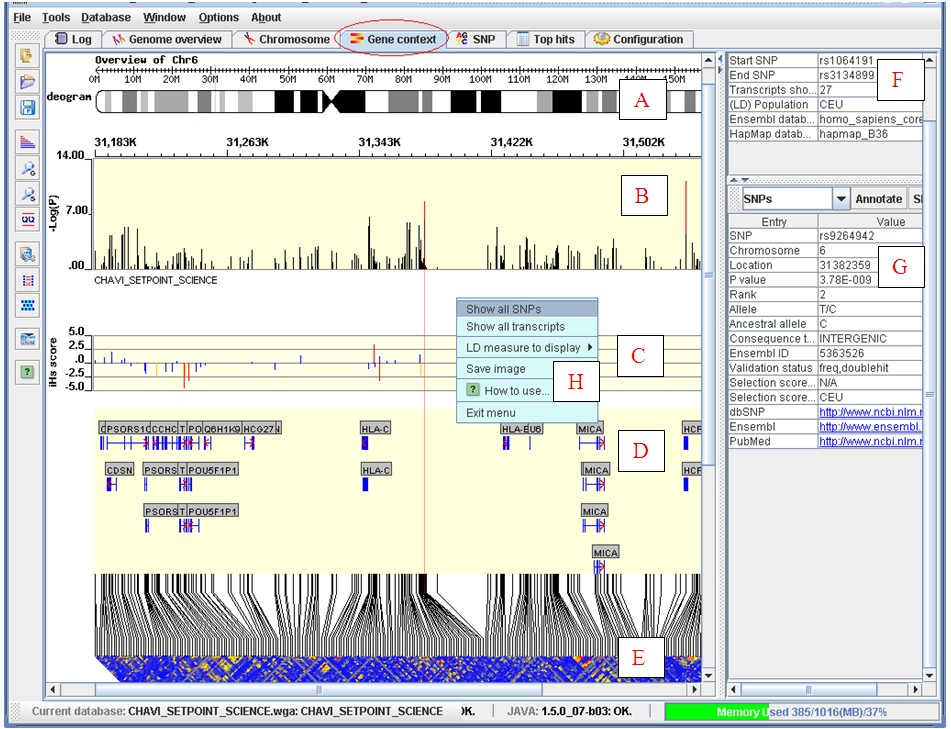
Figure 3.3.2.b-1. Results of comprehensive annotation for top hits: rs9264942, genic view. A: Chromosome ideogram; B: SNP P value lines; C: Recent selection score; D: transcripts; E: LD matrix; F: Description for annotated region; G: Dynamic data sheet; H: Popup menu. (Click to enlarge)
A: Chromosome ideogram : shows the annotated region on a chromosome with a transparent red rectangle;
B: Association results : show the SNPs with successful association P values. Different from chromosome view (3.3.2.a), these lines are spaced according to their actual physical location based on the latest genome build (Hubbard et al. 2007) . This panel will always plot every SNP P value line, no matter how many SNPs to be plotted, therefore the P value lines could be overlapped but the highest –LogP (lowest P value) can always be seen and be highlighted. Each SNP P value line will respond to mouse movement and will plot a red highlight line towards part D to show the detailed information for each SNP, together with the hyperlink to external databases, in an dynamic data sheet (part G); Click on each SNP line to bring up a resource menu (Figure 3.3.2.b-2). For lines too dense to easily pick up by mouse movement, press key “<”/”,” to move the highlighted lines backward (left, towards smaller chromosome coordinates), or key “>”/”.” to move the highlighted lines forward (right, towards larger chromosome coordinates), and then press key “enter” to bring up this menu.
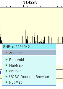
Figure 3.3.2.b-2. Resource menu for SNPs
C: Recent selection score (Voight et al. 2006) where available for SNPs shown in part B;
D: Transcripts : shows transcripts located in the annotated region. Exons are plotted as blue rectangles with a red arrow representing the strand. Each transcript will respond to mouse movement and will show the detailed information for each SNP, together with the hyperlink to external databases, in an dynamic data sheet (part G). Alternative transcripts are plotted with detailed exon information shown in the dynamic data sheet too (part G); Click on each transcript to bring up a resource menu (Figure 3.3.2.b-3). For transcripts too dense to easily pick up by mouse movement, press key “<”/”,” to move backward (left, towards smaller chromosome coordinates), or key “>”/”.” to move forward (right, towards larger chromosome coordinates), and then press key “enter” to bring up this menu.
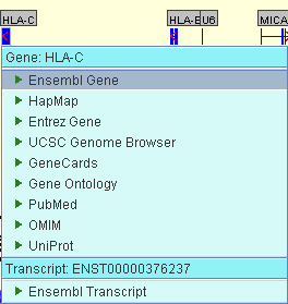
Figure 3.3.2.b-3. Resource menu for transcripts
E: LD matrix : shows the LD data (The International HapMap Consortium. 2005) among the SNPs plotted in part B. based on selected HapMap population. The r2 for the color scheme is: blue 0-0.2; yellow 0.2-0.6; red 0.6-1.0. Missing values are coded as -9 and plotted in gray. Each LD cell responds to mouse movement and will show detailed LD information, including the names of the two SNPs, r2 and D', together with HapMap population in the dynamic data sheet (part G);
F: Description for annotated region : shows the physical location and landmark for the start and end of the annotated region. The version of the Ensembl and HapMap databases are also shown in this data sheet. Differing from the dynamic data sheet (part G), the contents of this data sheet are fixed, unless other annotation results are selected. The coordinate discrepancies between the latest Ensembl and HapMap genome builds are adjusted automatically and the coordinates from the latest Ensembl databases are shown in all annotation reports. This enables an accurate alignment between Ensembl variation/transcript data and HapMap LD data.
G: Dynamic data sheet : shows the detailed information for the highlighted item in part B-E. Therefore the contents of this data sheet will change according to which type of item is highlighted in the main graphical region. This data sheet has also a fixed tool bar including a drop-down menu for all the SNPs shown in part B, sorted by the rs#. The user can select any SNP and show the detailed information in the dynamic data sheet. A red highlight line will also then be plotted on part B to D to show which SNP has been clicked. Sometimes this is more convenient than directly pointing the mouse to a specific SNP in part B, because when the SNP density is higher it is difficult to conveniently highlight a SNP among the overlapped lines. For SNP and transcript, this data sheet always offers hyperlinks to external databases, including Ensembl and NCBI, for a convenient reference for data not shown.
H: Popup menu : Clicking on blank region (other than hotspots, for example SNPs or transcripts) will activate this popup menu. It can then be dismissed by click on menu item “Exit”. This popup menu offers four functions:
H.1 Show all SNPs : click on this menu item will activate a popup window and show the detailed information for all the SNPs (Figure 3.3.2.b-4) plotted in part B, instead of one by one in dynamic data sheet (part G). This data sheet window offers four methods to sort the SNP collection: by location, by P value, by rs #, or by type. Select the sorting method and then click on button “Sort by”.

Figure 3.3.2.b-4. Results of comprehensive annotation for top hits: rs9264942, genic view, data sheet for showing all SNPs. (Click to enlarge)
Like the dynamic data sheet, this data sheet window also offers the clickable hyperlink navigating to dbSNP, Ensembl, and PubMed. In addition to this, if one clicks on rs# for each SNP, a red highlight line will be drawn on part B to D to indicate the location of the selected SNP. To dismiss this window, click on the “OK” button. The user also has the option to save the contents of this table to a comma separated text file (.csv) by clicking on the “Save” button, or to copy the tab-separated contents to system clip board by clicking on the “Copy” button and pasting the data into external software, for example, any text editor or Microsoft EXCEL.
H.2 Show all transcripts : clicking on this menu item will activate a popup window and show the detailed information for all the transcripts (Figure 3.3.2.b-5) plotted in part D, instead of one by one in dynamic data sheet (part G). This data sheet window offers up to six methods to sort the transcript collection: by location, by gene symbol (if available), by biotype (if available), by gene ontology (GO) term (if available), by Ensembl gene ID, or by Ensembl transcript ID. Select the sorting method and then click on button “Sort by”.

Figure 3.3.2.b-5. Results of comprehensive annotation for top hits: rs9264942, genic view, data sheet for showing all transcripts. (Click to enlarge)
Like the dynamic data sheet, this data sheet window also offers the clickable hyperlink navigating to the Ensembl transcript (and then to the Entrez Gene if needed), the Ensembl exon, and PubMed. To dismiss this window, click on the “OK” button. One also has the option to save the contents of this table to a comma separated text file (.csv) by clicking on the “Save” button, or to copy the tab-separated contents to the system clip board by clicking on the “Copy” button and pasting the data into external software, for example, any text editor or Microsoft EXCEL.
H.3 LD measures to display : click on this menu item to choose whether to display D' or r 2 in LD matrix.
H.4 Save image: click on this menu item to save the entire chromosome view panel as an image file (Figure 3.3.2.b-6). Four image formats are supported: bmp, jpg, png, or eps (for publishing).

Figure 3.3.2.b-6. Results of comprehensive annotation for top hits: rs9264942, genic view, save image. (Click to enlarge)
Next: Top hits annotation: SNP view